Theoretical approaching methodology

Flamant model

In Hertzian contact, the two contacting bodies are treated locally as elastic half‑spaces, and the fundamental solution is the stress field in a semi‑infinite solid due to surface tractions. One convenient way to build intuition is to start from a concentrated load acting on a straight boundary (edge) or on the surface of a semi‑infinite body, then generalize this to a load distributed over a finite contact area, which is exactly what Hertz contact does. Consider a semi-infinite elastic plate (half‑plane in 2D, half‑space in 3D) as shown in Fig.1.

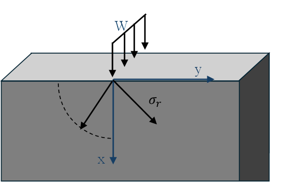
When a concentrated normal load, W,  is applied at the boundary point (x=0, y=0) 

, the resulting stress field σ(x,y) can be written in closed form using the classical Boussinesq (3D) or Flamant (2D) solutions, depending on whether you treat the problem as a half‑space or a half‑plane. In 2D (plane stress/plane strain, “concentrated load on a straight boundary” in the sense of a line load per unit thickness into the page), the Flamant solution for a vertical load, P,  at the edge gives stress components in polar coordinates (r,Θ) measured from the load application point along the boundary. These expressions represent your “concentrated load” case conceptually linked to equation (1); even if you do not explicitly write them in the paper, equation (1) is mathematically of this type: a stress field σ(x,y)  generated by a point (or line) load, P,  on the boundary of a semi-infinite elastic body.

Now, consider a normal load distributed over a finite region of the surface—along a segment of the boundary in the 2D (half-plane) case, or over an area in the 3D (half-space) case. Let the load distribution along the boundary be p(y) [force per unit length] at the point y (in 2D), such that the infinitesimal force applied over an infinitesimal segment p(y)dy. The stress at a point (x,y) in the semi-infinite plate due to this distributed load can then be written as the sum (or integral) of the infinitesimal stress contributions from each loaded segment. To simplify, let the sum of the load be P. The equation of radial stress can be defined below;

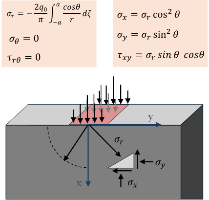
Utilizing transformation equation, the stress of of state of σx and σy

 expressed in terms of σr as below: